This post is also available as a github gist: afrendeiro/eb5b2ab723f89ed64eb81a28b2ad78c4
This post explores how to leverage spatial information for cell type prediction using two graph-based models: a Diffusion Classifier and a Graph Neural Network (GNN).
We will use squidpy for spatial data handling and scikit-network for the models, benchmarking their performance as the fraction of known cell type labels varies.
Setting Up: data and spatial graphs
First, we load a sample IMC (Imaging Mass Cytometry) dataset using squidpy and construct a spatial graph. This graph represents the proximity of cells, where nodes are cells and edges connect neighboring cells.
import squidpy as sq
import numpy as np
import pandas as pd
import matplotlib.pyplot as plt
from tqdm import tqdm

from sknetwork.classification import DiffusionClassifier
from sknetwork.gnn.gnn_classifier import GNNClassifier
from sknetwork.classification import get_accuracy_score, get_average_f1_score

figkws = dict(dpi=300, bbox_inches="tight")
np.random.seed(42)

# Load data and make spatial graph
a = sq.datasets.imc()
sq.gr.spatial_neighbors(a, n_neighs=10, coord_type="generic")
The models: Diffusion and GNN
We define a function predict_cell_types that takes an AnnData object, a fraction of cells to use as known labels, and the model family (“diffusion” or “gnn”). The function randomly samples a subset of cells whose labels are “known” to the model, simulating a semi-supervised learning scenario. It then trains the specified model and evaluates its accuracy and F1-score. A crucial aspect is the comparison against a “shuffled” baseline, where the known labels are randomly permuted. This helps ascertain if the models are truly leveraging spatial information or just fitting to random assignments.
- Diffusion classifier: This model propagates labels across the graph based on diffusion principles, where labels spread more strongly to closer, connected nodes. It does not take node features into account, focusing solely on the graph structure.
- GNN classifier: A Graph Neural Network learns to classify nodes by aggregating feature information from their neighbors, making it suitable for capturing complex relationships in spatial data.
def predict_cell_types(
    a, fraction: float = 0.5, model_family: str = "diffusion", **kwargs
) -> np.ndarray:
    """
    Predict cell types using diffusion based on known labels.
    """
    adj = a.obsp["spatial_connectivities"]
    features = a.X
    y = a.obs["cell type"].cat.codes

    n_classes = a.obs["cell type"].nunique()
    n_nodes = a.shape[0]
    n_known_labels = int(fraction * n_nodes)
    known_indices = np.random.choice(n_nodes, size=n_known_labels, replace=False)
    known_labels = {idx: y.iloc[idx] for idx in known_indices}

    shuffled_codes = np.random.permutation(a.obs["cell type"].cat.codes)
    shuffled_labels = {idx: shuffled_codes[idx] for idx in known_indices}

    if model_family == "diffusion":
        model = DiffusionClassifier(**kwargs)
        model.fit(adj, labels=known_labels)
        shuffled_model = DiffusionClassifier(**kwargs)
        shuffled_model.fit(adj, labels=shuffled_labels)
    elif model_family == "gnn":
        model = GNNClassifier(
            dims=int(n_classes),
            learning_rate=1e-1,
            patience=100,
            early_stopping=False,
            **kwargs,
        )
        model.fit(adjacency=adj, features=features, labels=known_labels)
        shuffled_model = GNNClassifier(
            dims=int(n_classes),
            learning_rate=1e-1,
            patience=100,
            early_stopping=False,
            **kwargs,
        )
        shuffled_model.fit(adjacency=adj, features=features, labels=shuffled_labels)

    pred = pd.Series(model.predict(), index=a.obs_names)
    a.obs["prediction"] = pred
    acc = get_accuracy_score(y, pred)
    avg_f1 = get_average_f1_score(y, pred)
    shuffled_pred = pd.Series(shuffled_model.predict(), index=a.obs_names)
    shuffled_acc = get_accuracy_score(y, shuffled_pred)
    shuffled_avg_f1 = get_average_f1_score(a.obs["cell type"].cat.codes, shuffled_pred)

    return dict(
        fraction=fraction,
        accuracy=acc,
        average_f1=avg_f1,
        shuffled_accuracy=shuffled_acc,
        shuffled_average_f1=shuffled_avg_f1,
    )
Benchmarking Performance with Subsampling
We now run the predict_cell_types function for both diffusion and GNN models across a range of fractions (from very small to 100% of cells known). This allows us to observe how the models’ performance scales with the amount of available ground truth data.
_res = list()
f = np.exp(np.linspace(1e-5, 1.0, 50))
f = (f - f.min()) / (f.max() - f.min())
for model_family in tqdm(["diffusion", "gnn"], position=0, leave=False, desc="Models"):
    for fraction in tqdm(f[1:], position=1, leave=False, desc="Fractions"):
        metrics = predict_cell_types(a, fraction=fraction, model_family=model_family)
        _res.append({"model_family": model_family} | metrics)
res = pd.DataFrame(_res)
res.to_csv("spatial_clustering_demo.subsampling_results.csv", index=False)
The results are then plotted to visualize the accuracy and average F1-score against the fraction of known cells:
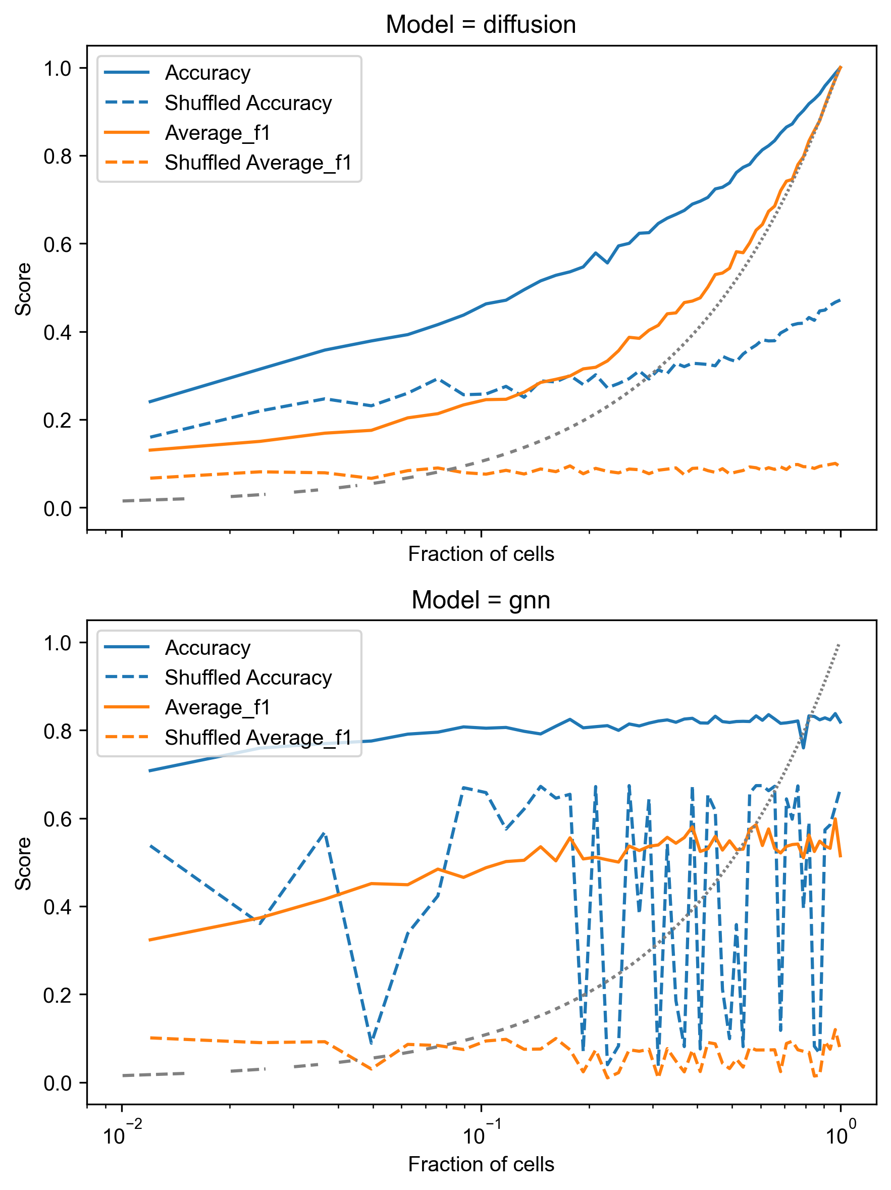
A few key trends:
- Performance improvement: Both Diffusion and GNN models show a clear increase in accuracy and F1-score as the fraction of cells with known labels increases. This is expected, as more training data generally leads to better performance.
- Superiority over shuffled baseline: For both models, the “Accuracy” and “Average F1” curves are consistently above their respective “Shuffled Accuracy” and “Shuffled Average F1” baselines. This indicates that the models are effectively leveraging the spatial information and not just random chance, especially at higher fractions of known cells.
- GNN performance: The GNN model appears to achieve higher accuracy and F1-scores, particularly at lower fractions of known cells. It also shows a steeper increase in performance, suggesting it can learn more complex spatial patterns from limited labels. However, its shuffled baseline also shows more variability, possibly due to the nature of GNN training with features.
- Diffusion performance: The Diffusion model shows a more stable performance curve, consistently improving with more data. While it might not reach the peak performance of the GNN in this specific setup, its smooth increase in performance relative to its shuffled baseline indicates robust learning from spatial proximity.
- Impact of limited data: At very low fractions of known cells (left side of the x-axis, which is log-scaled), the performance of both models is closer to the shuffled baseline, highlighting the challenge of predicting cell types with minimal supervision.
Visualizing Predictions
Finally, we visualize the predicted cell types on the spatial graph for two specific scenarios: when 20% and 50% of the cells have known labels. This provides a qualitative understanding of how well the models reconstruct the true cell type distribution.
# Visualize predictions with 50% cells
for fraction in [0.2, 0.5]:
    perc = f"{int(fraction * 100):02d}%"
    fig, axes = plt.subplots(2, 2, figsize=(2 * 6, 2 * 6))
    sq.pl.spatial_scatter(a, shape=None, color="cell type", fig=fig, ax=axes[0][0])
    r0 = predict_cell_types(a, fraction=fraction, model_family="diffusion")
    a.obs["prediction"] = a.obs["prediction"].astype("category")
    sq.pl.spatial_scatter(a, shape=None, color="prediction", fig=fig, ax=axes[1][0])
    r1 = predict_cell_types(a, fraction=fraction, model_family="gnn")
    a.obs["prediction"] = a.obs["prediction"].astype("category")
    sq.pl.spatial_scatter(a, shape=None, color=["prediction"], fig=fig, ax=axes[1][1])
    axes[0, 0].set(title="Ground truth: Cell type")
    axes[0, 1].axis("off")
    axes[1, 0].set(
        title=f"Diffusion model w/ {perc} cells\nAccuracy: {r0['accuracy']:.2f}, F1: {r0['average_f1']:.2f}"
    )
    axes[1, 1].set(
        title=f"GNN w/ {perc} cells\nAccuracy: {r1['accuracy']:.2f}, F1: {r1['average_f1']:.2f}"
    )
    fig.savefig(f"spatial_clustering_demo.subsampling_results.{perc}.png", **figkws)
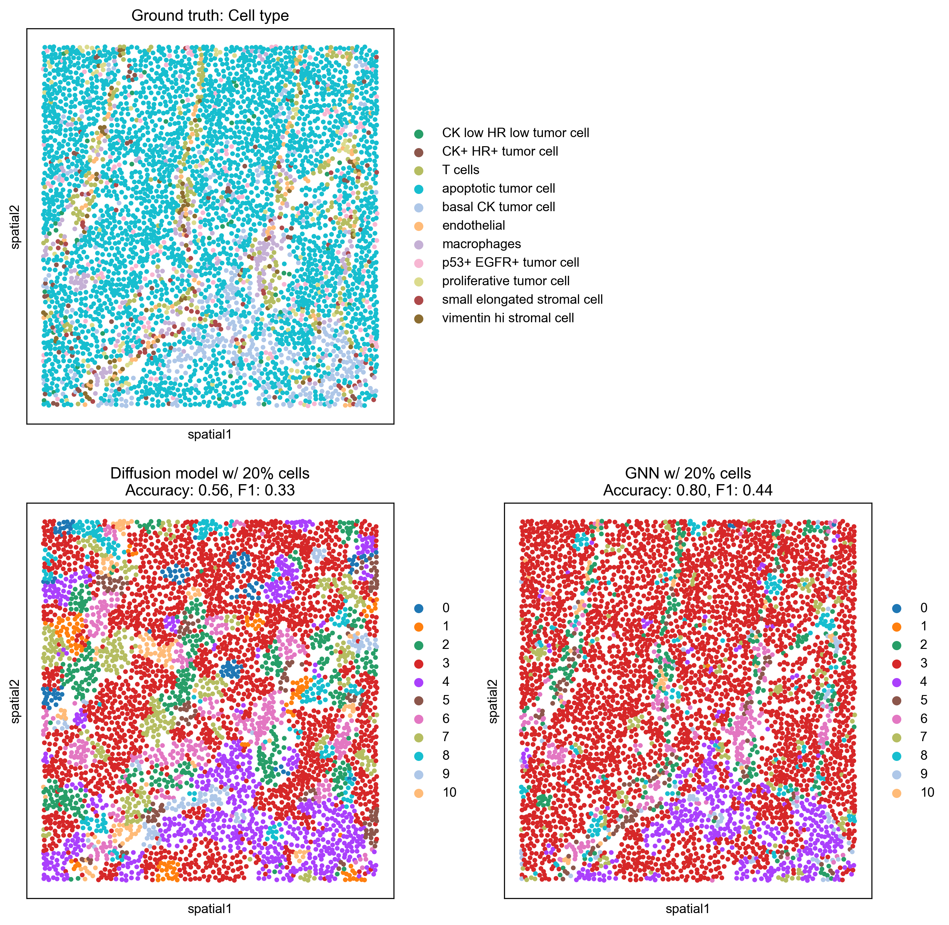
With 20% known cells, the GNN model (Accuracy: 0.80, F1: 0.44) visually outperforms the Diffusion model (Accuracy: 0.56, F1: 0.33), showing a more coherent capture of the ground truth spatial patterns.
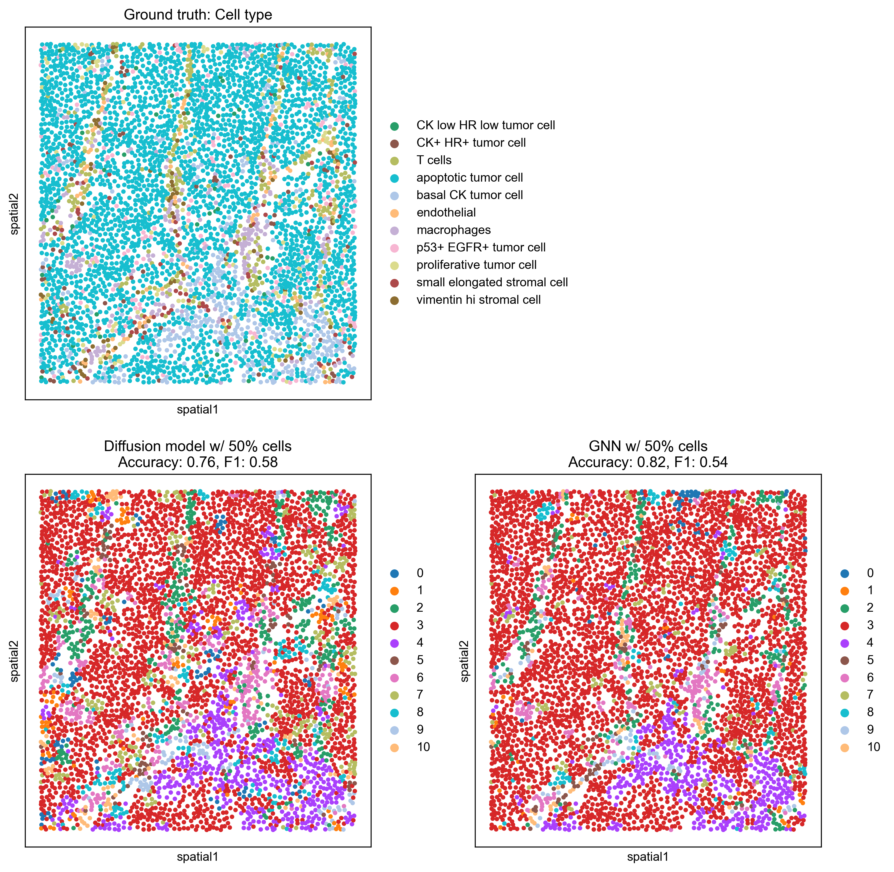
With 50%, both models show significant improvement. The GNN (Accuracy: 0.82, F1: 0.54) continues to produce predictions that closely resemble the ground truth. The Diffusion model (Accuracy: 0.76, F1: 0.58) also improves substantially, with its F1-score becoming comparable to the GNN, indicating better balance in its predictions.
Conclusion
This demo highlights the effectiveness of graph-based models, such as Diffusion Classifiers and Graph Neural Networks, for cell type prediction in spatial transcriptomics data. By leveraging spatial relationships, these models can infer cell types even with limited ground truth labels. The benchmarking results and spatial visualizations underscore the importance of spatial context for accurate biological interpretation and show how performance improves with increasing amounts of labeled data. Crucially, the inclusion of “shuffled” models provides a vital baseline, confirming that the observed performance gains are indeed due to the models learning meaningful spatial relationships rather than merely fitting to random label distributions.
It’s notable that the GNN, which explicitly accounts for cell features, generally performs better in this case than the Diffusion model, which does not. This improved performance comes with the trade-off of requiring considerably more effort for hyperparameter tuning. While allowing some overfitting might be acceptable for a single sample demonstration, real-world applications would need careful tuning to ensure robustness.
In a practical scenario, a similar approach could be used with a matched set of phenotyped cells to predict the identity of other, lower-quality ones. Although this example uses random spatial subsampling, which differs from the non-random spatial distribution of low-coverage cells that might be found in real-world datasets, the method could still prove valuable.