I’m interested in exploring flow cytometry data from a single-cell perspective. After all it is a very high throughput method that can measure a modest amount of variables in each single cell.
I decided to use the FlowCytometryTools Python library just to see what I could extract from those magic fcs files and how feature complete the library is.
I made the following Jupyter notebook:
Demo of exploring flow cytometry data with the FlowCytometryTools library
# Import library
from FlowCytometryTools import FCMeasurement
# load fcs file (version 3)
sample = FCMeasurement(ID='Example sample', datafile="data/example.fcs")# Let's see the number of cells measured
sample.counts156157
# All metadata
sample.meta.items()[:10] # see only first 10 entries
[(u'P13MS', u'350'),
(u'$ETIM', u'13:21:42'),
(u'P8DISPLAY', u'LOG'),
(u'FSC ASF', u'0.74'),
(u'CYTNUM', u'1'),
(u'$ENDDATA', u'9998405 '),
(u'P2DISPLAY', u'LIN'),
(u'$ENDSTEXT', u'0'),
(u'LASER2NAME', u'Red')]
sample.channel_names(u'FSC-A',
u'FSC-H',
u'FSC-W',
u'SSC-A',
u'SSC-H',
u'SSC-W',
u'B/E Alexa Fluor 488-A',
u'B/C PE-TexasRed-A',
u'B/B PerCP-Cy5-5-A',
u'YG/A PE-Cy7-A',
u'R/C APC-A',
u'R/B Alexa Fluor 700-A',
u'R/A APC-Cy7-A',
u'V/C Pacific Blue-A',
u'YG/E PE-A',
u'Time')
sample.channels| $PnN | $PnB | $PnG | $PnE | $PnR | $PnV | |
|---|---|---|---|---|---|---|
| Channel Number | ||||||
| 1 | FSC-A | 32 | 1.0 | [0, 0] | 262144 | 244 |
| 2 | FSC-H | 32 | 1.0 | [0, 0] | 262144 | 244 |
| 3 | FSC-W | 32 | 1.0 | [0, 0] | 262144 | 244 |
| 4 | SSC-A | 32 | 1.0 | [0, 0] | 262144 | 276 |
| 5 | SSC-H | 32 | 1.0 | [0, 0] | 262144 | 276 |
| 6 | SSC-W | 32 | 1.0 | [0, 0] | 262144 | 276 |
| 7 | B/E Alexa Fluor 488-A | 32 | 1.0 | [0, 0] | 262144 | 469 |
| 8 | B/C PE-TexasRed-A | 32 | 1.0 | [0, 0] | 262144 | 450 |
| 9 | B/B PerCP-Cy5-5-A | 32 | 1.0 | [0, 0] | 262144 | 462 |
| 10 | YG/A PE-Cy7-A | 32 | 1.0 | [0, 0] | 262144 | 458 |
| 11 | R/C APC-A | 32 | 1.0 | [0, 0] | 262144 | 586 |
| 12 | R/B Alexa Fluor 700-A | 32 | 1.0 | [0, 0] | 262144 | 560 |
| 13 | R/A APC-Cy7-A | 32 | 1.0 | [0, 0] | 262144 | 618 |
| 14 | V/C Pacific Blue-A | 32 | 1.0 | [0, 0] | 262144 | 385 |
| 15 | YG/E PE-A | 32 | 1.0 | [0, 0] | 262144 | 443 |
| 16 | Time | 32 | 0.01 | [0, 0] | 262144 | None |
# get forward vs side scatter of first 10 cells
sample.data[['FSC-A', 'SSC-A']][:10]| FSC-A | SSC-A | |
|---|---|---|
| 0 | 53618.921875 | 42435.988281 |
| 1 | 100054.664062 | 33288.808594 |
| 2 | 60825.039062 | 35168.011719 |
| 3 | 58227.640625 | 37189.890625 |
| 4 | 67312.617188 | 39781.621094 |
| 5 | 92615.437500 | 73334.914062 |
| 6 | 51280.519531 | 33090.449219 |
| 7 | 43725.859375 | 36683.550781 |
| 8 | 62111.902344 | 22713.960938 |
| 9 | 84667.843750 | 33091.320312 |
# Get all channels in one table
# this would be the main table to work on from here
sample.data.drop("Time", axis=1).head(10) # show only first 10 cells| FSC-A | FSC-H | FSC-W | SSC-A | SSC-H | SSC-W | B/E Alexa Fluor 488-A | B/C PE-TexasRed-A | B/B PerCP-Cy5-5-A | YG/A PE-Cy7-A | R/C APC-A | R/B Alexa Fluor 700-A | R/A APC-Cy7-A | V/C Pacific Blue-A | YG/E PE-A | |
|---|---|---|---|---|---|---|---|---|---|---|---|---|---|---|---|
| 0 | 53618.921875 | 46566.0 | 75462.132812 | 42435.988281 | 40018.0 | 69495.859375 | 66.989998 | 59.160000 | 36.540001 | 5453.760254 | 2175.400146 | 624.150024 | 329.960022 | 9.130000 | 156.400009 |
| 1 | 100054.664062 | 90369.0 | 72560.093750 | 33288.808594 | 32241.0 | 67665.867188 | 62.639999 | 215.759995 | 97.440002 | 2553.920166 | 2539.670166 | 579.619995 | 252.580002 | 14.940000 | 720.359985 |
| 2 | 60825.039062 | 53044.0 | 75149.492188 | 35168.011719 | 33952.0 | 67883.210938 | 90.480003 | 125.279999 | 28.710001 | 6724.280273 | 1590.670044 | 669.410034 | 292.000000 | 6.640000 | 291.640015 |
| 3 | 58227.640625 | 50084.0 | 76192.140625 | 37189.890625 | 35568.0 | 68524.421875 | 69.599998 | 334.950012 | 139.199997 | 2679.040039 | 1762.950073 | 458.440002 | 202.210007 | 9.960000 | 917.239990 |
| 4 | 67312.617188 | 57849.0 | 76257.140625 | 39781.621094 | 38333.0 | 68012.632812 | 77.430000 | 192.270004 | 100.919998 | 4035.120117 | 1524.970093 | 475.230011 | 239.440002 | 9.960000 | 608.119995 |
| 5 | 92615.437500 | 72473.0 | 83750.437500 | 73334.914062 | 66461.0 | 72314.242188 | 120.059998 | 2424.689941 | 2306.370117 | 253.919998 | 237.980011 | 241.630005 | 66.430000 | 34.029999 | 6612.040039 |
| 6 | 51280.519531 | 44760.0 | 75083.117188 | 33090.449219 | 31656.0 | 68505.679688 | 86.129997 | 57.420002 | 32.189999 | 2461.920166 | 1025.650024 | 365.000000 | 151.839996 | 43.989998 | 80.040001 |
| 7 | 43725.859375 | 38597.0 | 74244.570312 | 36683.550781 | 35153.0 | 68389.421875 | 153.990005 | 202.710007 | 163.559998 | 2104.040039 | 1400.140015 | 401.500000 | 234.330002 | 191.729996 | 734.160034 |
| 8 | 62111.902344 | 55068.0 | 73918.890625 | 22713.960938 | 21820.0 | 68221.000000 | 73.080002 | 46.110001 | 81.779999 | 4808.839844 | 1565.119995 | 646.049988 | 348.940002 | 12.450000 | 123.279999 |
| 9 | 84667.843750 | 75601.0 | 73395.750000 | 33091.320312 | 32645.0 | 66432.007812 | 31.320000 | 15.660000 | 13.050000 | 3248.520020 | 1015.430054 | 360.619995 | 141.620010 | 6.640000 | 75.440002 |
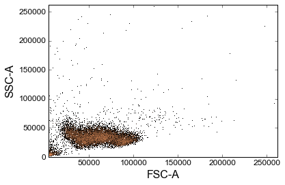
# Let's plot some things:
# plot with provided library wrappers
_ = sample.plot(['FSC-A', 'SSC-A'], bins=1000)
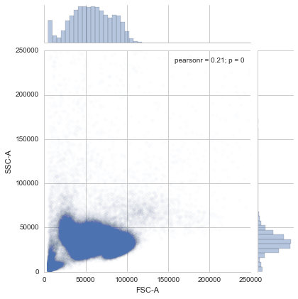
# we can obviously also plot with base matplotlib + seaborn
import matplotlib.pyplot as plt
import pylab
import seaborn as sns
sns.set_style("whitegrid")
sns.jointplot(sample.data['FSC-A'], sample.data['SSC-A'],
xlim=(0, 250000), ylim=(0, 250000),
alpha=0.01)<seaborn.axisgrid.JointGrid at 0x7f334e8f0b50>
# Now let's make a gate using the interactive interface
# sample.view_interactively()
from FlowCytometryTools import ThresholdGate, PolyGate
# Four threshold gates
gate1 = ThresholdGate(17500, 'FSC-A', region='above')
gate2 = ThresholdGate(60000, 'SSC-A', region='below')
gate3 = ThresholdGate(110000, 'FSC-A', region='below')
gate4 = ThresholdGate(10000, 'SSC-A', region='above')
# Similar thing with a polygon
# drawn interactively
gate5 = PolyGate(
[(3.140e+04, 9.951e+04), (1.108e+04, 5.092e+04), (1.421e+04, 3.304e+04),
(2.385e+04, 2.426e+04), (3.219e+04, 1.583e+04), (3.818e+04, 5.706e+03),
(5.251e+04, 4.019e+03), (1.208e+05, 1.178e+04), (1.408e+05, 5.429e+04),
(3.505e+04, 9.681e+04), (3.114e+04, 9.951e+04), (3.219e+04, 9.613e+04)],
('FSC-A', 'SSC-A'), region='in', name='gate4')
_ = sample.plot(['FSC-A', 'SSC-A'], bins=1000, gates=[gate1, gate2, gate3, gate4, gate5])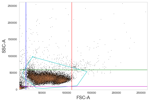
# Plot channels individually
_ = sample.plot('FSC-A', bins=1000)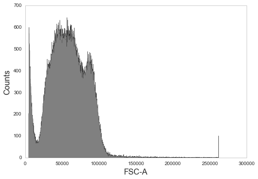
# Log transform and plot again
_ = sample.transform('hlog', channels=['FSC-A']).plot('FSC-A', bins=1000)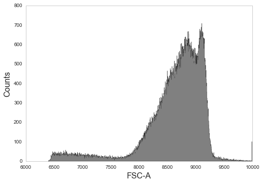
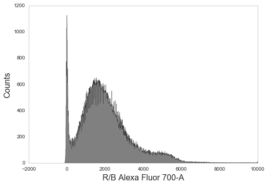
# Log transform and plot different channel
_ = sample.transform('hlog', channels=['R/B Alexa Fluor 700-A']).plot('R/B Alexa Fluor 700-A', bins=1000)